Statistical Test Of Commodore And Radio Shack RND
Brian Flynn
This article provides a statistical test of the randomness of your BASIC'S random number generator. Versions of the program for TRS–80 Color Computers with Extended Color BASIC and for PET/CBM, VIC, and 64 computers are provided. To use the TRS-80 version with non-Extended BASIC, you must substitute the value of square root of N for SQR(N) in lines 6110 and 6120, since non-Extended Color BASIC has no square root function. (SQR(1000) = 31.6228.) Alternatively, the Color BASIC manual lists a square root routine on page 116. The only changes necessary to use the PET/CBM version on the VIC-20 or Commodore 64 are to adapt the PRINT statements to the smaller screen sizes.
As presented, the program takes several hours to sort each subsequence. Thus, several days would be required for a complete program run. Each of the following options significantly reduces the required execution time:
- Replace the sort routine (Module 5) with a faster sorting routine. (See "All Sorts of BASIC Sorts," COMPUTE!, December 1982, #31.)
- Compile the program before running it. (Of course, to do this you must have a BASIC compiler.)
- Reduce the number of fractions specified in the DATA statement of line 2020.
The phrase "Kolmogorov-Smirnov" brings to mind the vision of a big white dog, a beautiful princess, and a bearded, virile, vodka-drinking czar. In reality, however, "Kolmogorov-Smirnov" is not this imaginary troika from pre-Bolshevik days, but rather a statistical test, named after two Russian mathematicians, for trying to determine how well values from a sample match values from a specified population.
The test is often used to examine the degree of randomness of sequences of fractions generated by the computer from a uniform distribution. This article explains the Kolmogorov-Smirnov test in more detail, and then uses the test to evaluate the quality of the random number generator in Microsoft's BASIC compiler for the TRS-80 and Commodore computers.
Kolmogorov-Smirnov Test
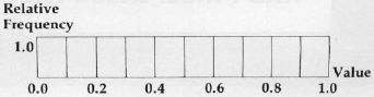
The command "RND(O)" in TRS-80 BASIC generates a fraction from a uniform distribution between 0 and 1, exclusive. In this distribution, graphed in Figure 1, the probability of drawing a fraction between 0.0 and 0.1, in a one-shot selection, is equal to the probability of drawing a fraction between 0.1 and 0.2, or 0.2 and 0.3, and so on. In each case, the probability is 1/10 since the distribution is divided into ten equal parts.
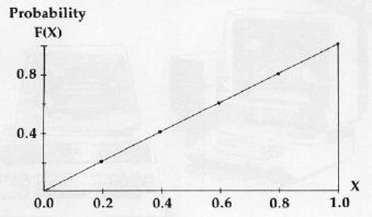
Now, the Kolmogorov-Smirnov test uses cumulative rather than absolute relative frequency distributions. Referring again to the uniform distribution of Figure 1, note that the probability of drawing a fraction less than or equal to 0.2 is 1/10 + 1/10, or 0.2. Similarly, the probability of drawing a fraction less than or equal to 0.3 is 1/10 + 1/10 + 1/10, or 0.3. In general, the probability of selecting a fraction less than or equal to some number X is simply X, where X ranges from 0 to 1. The distribution based upon these cumulative probabilities is graphed in Figure 2.
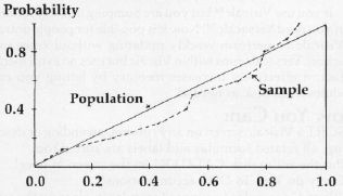
The essence of the Kolmogorov-Smirnov test is comparing theoretical and empirical cumulative frequency distributions. An example of the latter type of distribution is based upon the following sequence of ten fractions, rounded to three decimal places, generated by executing "RND(0)" on a Honeywell computer: 0.789, 0.528, 0.871, 0.097, 0.276, 0.434, 0.711, 0.535, 0.776, and 0.918. If the sample sequence is random, then the empirical cumulative frequency distribution, based upon observed values sorted in ascending order, should approximate the theoretical one. These distributions are compared in Table 1 and Figure 3.
These two displays reveal that the observed fractions are a little too high, and that the empirical distribution is therefore a little too low. But is it so low that we reject the null hypothesis of a random sequence? The following two test statistics are used to answer this question (Professor Knuth, p. 45):
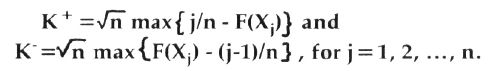
The symbol K+ is the maximum vertical distance between the two curves when the empirical distribution is higher than the theoretical distribution, and K- is the maximum distance when the empirical distribution is lower. Further, n is the sample size, ten in this case. And F(Xj) is the theoretical cumulative frequency for the jth observation. For example, F(X1) = 0.097 since 9.7% of all values from a uniform distribution are ≤ 0.097. Similarly, F(X2) = 0.276, and so on.
For our data, K+= 0.259 and K- = 0.740. Referencing Kolmogorov-Smirnov critical values (Professor Knuth, p. 44), both of these statistics fall in the acceptance region for the null hypothesis at the 10% level of significance, using a two-tail test (5% of the distribution's area is under each tail). Hence, we can't label the observed sequence of fractions "nonrandom."
A Practical Application
The quality of the random number generator in Microsoft's BASIC is examined here, using the computer program listed at the end of the article. Specifically, the degree of randomness of the sequence of the first 50,000 fractions generated by RND(0) is investigated. This is done by performing the Kolmogorov-Smirnov test on each successive interval of 1,000 fractions within the total sequence. Hence, 50 values of the K+ statistic and 50 values of the K- statistic are tallied.
Test results, summarized in Table 2, reveal that the K+ and K- values always fall within the middle 98 percentile portion of the distribution. And they fall within the middle 90 percentile part 92 out of 100 times. These results suggest that the random number generator is a good one.
As an additional check, however, the Kolmogorov-Smirnov test is applied once again, this time to the 50 K+ values and to the 50 K- values from before. As Professor Knuth indicates (p. 45), this enables us "... to detect both local and global nonrandom behavior." Test results, using
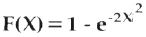
as the cumulative frequency distribution for the K values, are:
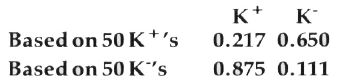
In all four cases, the null hypothesis of a random sequence is not rejected at the 2% level of significance, in a two-tail test. At the 10% level of significance Ho is rejected one out of four times, with 0.111 the guilty value.
The Kolmogorov-Smirnov test is useful in examining the randomness of sequences of fractions generated by RND(0). But remember, no random number generator is perfect. And just because a sequence passes one statistical test does not mean that it will pass a second.
References
Knuth, Donald E. The Art of Computer Programming, Vol. 2. Reading: Addison-Wesley Publishing Company, Inc., 1971.
Lapin, Lawrence L. Statistics for Modern Business Decisions. New York: Harcourt Brace Jovanovich, Inc., 1973, pp. 422-426.
Table 1: Sample And Theoretical Cumulative Relative Frequencies
| Fraction | Sample Cumulative Frequency | Theoretical Cumulative Frequency |
| 0.097 | 0.1 | 0.097 |
| 0.276 | 0.2 | 0.276 |
| 0.434 | 0.3 | 0.434 |
| 0.528 | 0.4 | 0.528 |
| 0.535 | 0.5 | 0.535 |
| 0.711 | 0.6 | 0.711 |
| 0.776 | 0.7 | 0.776 |
| 0.789 | 0.8 | 0.789 |
| 0.871 | 0.9 | 0.871 |
| 0.918 | 1.0 | 0.918 |
Note that the theoretical cumulative frequency always equals the value of the observed fraction. This is because the probability of drawing a fraction less than or equal to, say, 0.276, is 0.276, where the population is the uniform distribution between 0 and 1.
Table 2: Kolmogorov-Smirnov Test Results
Ho: The sequence is random
HA: The sequence is nonrandom
| Number Of Times In 50 Trials That Ho Is Rejected | ||||
| Level Of Significance | Critical Lower | Values Upper | K+ | K- |
| 2% | 0.066 | 1.511 | 0 | 0 |
| 10% | 0.156 | 1.219 | 4 | 4 |
| 50% | 0.375 | 0.828 | 26 | 26 |
Note: The level of significance is the probability of rejecting Ho when Ho is in fact true.
Figure 1. Uniform Distribution Between 0 And 1