Amiga Math Graphics
Warren Block
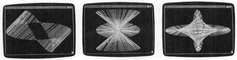
Is math boring? Before you answer, take a look at this Amiga BASIC program. It creates graceful, multicolored graphic designs based on a variety of interesting mathematical functions.
As one of my first Amiga programming projects, I decided to convert several Apple II+ hi-res graphics routines to run on my new machine. Originally, all these routines were written as one-liners: That is, the entire program would fit (just barely, sometimes) on one BASIC line. "Amiga Math Graphics" combines all of them into a single program. At the very least, these routines demonstrate the speed and power of the Amiga, while creating a pleasing visual display. At their best, perhaps they will convince you to explore the field of microcomputer graphics—a field which many people avoid because it seems difficult. Pictures are a fundamental part of communication, and being able to use graphics on the computer will improve your ability to communicate through that medium.
Type in the program and save a copy before you run it. The small ← character indicates where each program line ends. Don't try to type this character—we deliberately chose one that's not on the Amiga keyboard. The ← character merely shows where you should press RETURN to end one program line and start another.
Labeled Subroutines
Although the routines in this program were originally one-liners, it seemed a shame to keep them that way when AmigaBASIC makes it so easy to write neat, readable code. Each routine is marked with a descriptive label. Let's look at each of them in turn.
RightOvals. The basic formula used in this routine forms the basis for several different plotting routines. They all involve drawing a line from the perimeter of one oval to the perimeter of another. In this case, the line is drawn from a point on the first oval to a point halfway along the other.
SideOvals. Only minor changes were made to RightOvals to produce this interesting display. The second oval was tilted with respect to the first, and the line is plotted with an offset added to the x coordinate of the second oval.
Scaling Graphic Shapes
When the trigonometric functions sine and cosine are used for graphics, a problem arises because both of these functions return only values between 0 and 1. Without scaling (adjusting) the figures to fit the computer's display, you would see only three or four pixels in the middle of the screen. Scaling the display involves multiplying a set of coordinates by a constant amount. However, if you multiply both the x (horizontal) and y (vertical) coodinates by the same amount, the graph appears to be squashed horizontally on the screen. This occurs because the Amiga's aspect ratio (the ratio of horizontal to vertical pixels) is greater than 1. In plain English, there are more pixels across the screen than there are from top to bottom. To adjust for the aspect ratio, you must make the horizontal scaling factor larger than the vertical factor.
Other factors influence aspect ratio, including the type of monitor you have and the physical shape and relative locations of the pixels it displays. Some experimentation is required to find the best scaling values for any given display. In this program, the R variables (R1, R2, and so on) set the scaling factors for various routines. By changing these values, you can squash the shapes vertically or horizontally.
TwistedBand. Using a minor variation on the double-oval effect, this routine creates a display that looks remarkably like a twisted loop of paper. The only real difference from SideOvals is that an offset is added to the y coordinate of the second oval, not to its x coordinate.
Multilobe. This routine employs a common polar function which involves multiplying an angle theta by a fixed constant, then using this new value to compute the R value (theta and R are discussed at the end of this article). The effect is that of several squashed, distorted lobes instead of a plain circle. By setting the variable Lobes to 4, eight lobes are drawn. Try changing Lobes to different values (including nonintegers) for some interesting variations.
Show Your Colors
Before you bought an Amiga, you may have heard that it can display 4096 different colors. The low-resolution graphics screen lets you display as many as 32 different colors at once. If you're familiar with earlier computers, the Amiga's color system may seem confusing at first. On a Commodore 64, for example, color 2 is always red, and so on. But the Amiga, like the PC/PCjr, allows you to assign any color to color 2. The PALETTE statement allows you to define color 2 as black, magenta, or whatever you like. The color number simply provides a means for refering to that color—however you define it.
To use PALETTE, imagine that you have three cans of paint: one red, one green, and one blue. By mixing various portions of these cans together, you can create almost any conceivable color. For example, to make a bright red, take 90 percent of the paint in the red can and mix it with 20 percent of the paint in the green can (you don't need any blue). By coincidence, this is just the way the PALETTE statement works. The statement PALETTE 5,.90,.20,0 assigns a bright red color to color 5. (Strictly speaking, color mixing in Amiga BASIC is more like mixing colors of light than colors of paint. Thus, the statement PALETTE 5, 1, 1, 1 sets red, green, and blue to maximum intensity, creating a white color. If you mix red, green, and blue pigments of equal intensities, the result is a very dark brown or black.)
SpiralCone. Using a method similar to Multilobe, this routine multiplies the theta value by 3, resulting in a six-lobed figure. However, only the x coordinate for this figure is used. The y coordinate is calculated using the normal value of theta. A conelike shape is formed by drawing all lines from the center of the display to the calculated points.
SideSpiralCone. This is merely SpiralCone drawn sideways, with different scaling values. The difference in appearance is substantial enough to prevent most viewers from detecting the similarities.
The last two routines in the program rely on similar functions, but produce patterns that look very different on the screen.
Circles. This routine defines a small circle surrounded by a larger one; then it picks 6 equally spaced points on the inner circle. The final design is created by drawing a line from each of those points to 20 or so equally spaced points on the outer circle.
Spikes. Although this routine looks nearly identical to Circles, the shape it draws is completely different.
There's A System To This
You can enjoy and experiment with this program without understanding the math that underlies the graphics. For those who are interested, here's a further explanation of how it works.
In the field of mathematics, there are many systems for expressing the location of a point in a plane. Generally, the center of the system is referred to as the origin. The origin is simply a reference point; the location of all other points is defined with respect to the origin.
Most people are familiar with the Cartesian coordinate system, in which the location of any point is expressed in terms of x and y coordinates. The x value represents the point's horizontal distance from the point of origin. Similarly, the y coordinate represents the point's vertical distance from the origin.
The Cartesian system works well for representing two- and three-dimensional shapes on a two-dimensional surface such as the computer's display screen. However, the polar coordinate system is much more convenient when you're using trigonometric functions such as sine and cosine. In this scheme, a point's location is expressed as a distance from the origin (conventionally labeled R) and an angle (usually labeled theta, or with the Greek letter θ) from a reference line.
Polar Functions
The routines in this program are all based on polar functions. Since Amiga BASIC commands use Cartesian coordinates (roughly—see below), it's necessary to convert from polar to Cartesian coordinates. In general, this operation can be performed by the expressions X = R * COS(theta) and Y = R * SIN (theta).
There are a few difficulties in adapting the graph of a polar function to a computer display. The easiest problem to allow for is the fact that most graphics displays (including the Amiga's) use an upside-down Cartesian system: That is, a point's y coordinate specifies how far down the screen the point lies—the exact opposite of the normal Cartesian system. Since all of our shapes are vertically symmetrical, this problem can simply be ignored.
Another difficulty arises because the Amiga's display does not allow for negative coordinates. The Amiga's origin point is in the upper left corner of the screen, not the center of the viewing area as in the Cartesian system. This can easily be corrected by considering the middle of the display to be the origin. In the calculations, all this involves is adding an x and y offset to the points you wish to plot.
Amiga Math Graphics
MathGraphics:
GOSUB Initialize
' Repeat until the user presses a key.
WHILE INKEY$ = ""
' Module 1 : RightOvals
R1 = 150
R2 = 25
R3 = 25
R4 = 85
Inc = Pi/64
FOR Theta = 0 TO 2 * TwoPi STEP Inc
X1 = FNPolarX(R1, Theta)
Y1 = FNPolarY(R2, Theta)
X2 = FNPolarX(R3, Theta + Pi)
Y2 = FNPolarY(R4, Theta + Pi)
LINE(X2, Y2)-(X1, Y1), INT(RND * 31) + 1
NEXT
Pause
' Module 2 : SideOvals--
' Same thing, only different.
R1 = 150
R2 = 35
R3 = 65
R4 = 85
Inc = Pi/64
Offset = Pi/3
FOR Theta = 0 TO 3 * TwoPi STEP Inc
X1 = FNPolarX(R1, Theta)
Y1 = FNPolarY(R2, Theta)
X2 = FNPolarX(R3, Theta + Offset)
Y2 = FNPolary(R4, Theta)
LINE(X1, Y1)-(X2, Y2), INT(RND * 31) + 1
NEXT
Pause
' Module 3 : TwistedBand
' Yet another variation on the double oval theme.
R1 = 150
R2 = 35
R3 = 65
R4 = 85
Inc = Pi/64
offset = Pi/3
FOR Theta = 0 TO 3 * TwoPi STEP Inc
X1 = FNPolarX(R1, Theta)
Y1 = FNPolary(R2, Theta)
X2 = FNPolarX(R3, Theta)
Y2 = FNPolarY(R4, Theta + Offset)
LINE(X1, Y1)-(X2, Y2), INT(RND * 31) + 1
NEXT
Pause
' Module 4 : Multilobe
R1 = 100
Inc = Pi/128
Lobes = 4
FOR Theta = 0 TO 2 * TwoPi STEP Inc
R2 = R1 * SIN (Lobes * Theta)
X1 = FNPolarX(R2, Theta)
Y1 = FNPolary(R2, Theta)
LINE (XCenter, YCenter)-(X1, Y1), INT(RND * 31) + 1
NEXT
Pause
' Module 5 : Spiralcone
R1 = 100
R2 = 85
Inc = Pi/160
Lobes = 3
FOR Theta = 0 TO 2 * TwoPi STEP Inc
X1 = FNPolarX (R1, Theta * Lobes)
Y1 = FNPolarY (R2, Theta)
LINE (XCenter, YCenter)-(X1, Y1), INT(RND * 31) + 1
NEXT
Pause
' Module 6 : SideSpiralCone
R1 = 130
R2 = 80
Inc = Pi/160
Lobes = 3
FOR Theta = 0 TO 2 * TwoPi STEP Inc
X1 = FNPolarX(R1, Theta)
Y1 = FNPolarY(R2, Theta * Lobes)
LINE (XCenter, YCenter)-(X1, Y1), INT (RND * 31) + 1
NEXT
Pause
' Module 7 : Circles
R1 = 115
R2 = 85
R3 = 40
R4 = 45
Inc1 = Pi/3
Inc2 = Pi/20
For Theta1 = 0 To TwoPi STEP Inc1
For Theta2 = 0 To TwoPi STEP Inc2
X1 = FNPolarX(R1, Theta2)
Y1 = FNPolarY(R2, Theta2)
X2 = FNPolarX(R3, Theta1)
Y2 = FNPolarY(R4, Theta1)
LINE (X1, Y1)-(X2, Y2), INT(RND * 31) + 1
NEXT
NEXT
Pause
' Module 8 : Spikes
R1 = 115
R2 = 85
R3 = 40
R4 = 45
Inc1 = Pi/3
Inc2 = Pi/18
For Thetal = 0 To TwoPi STEP Inc1
For Theta2 = 0 To TwoPi STEP Inc2
X1 = FNPolarX(R1, Theta2)
Y1 = FNPolarY(R2, Theta1)
X2 = FNPolarX(R3, Theta1)
Y2 = FNPolarY(R4, Theta2)
LINE (X1, Y1)-(X2, Y2), INT(RND * 31) + 1
NEXT
NEXT
Pause
WEND
' Shut everything down and quit.
WINDOW CLOSE 2
SCREEN CLOSE 2
WINDOW OUTPUT 1
END
SUB Pause STATIC
FOR Delay = 1 TO 5000
NEXT
CLS
END SUB
Initialize : 4
' Set up a 32 color low-res screen.
SCREEN 2, 320, 200, 5, 1
WINDOW 2, "AmigaBASIC Graphics", (0, 0)-(297, 185), 23, 2
CLS
' Color 0 (background) is black.
PALETTE 0, 0, 0, 0
' Set up the other 31 colors as random combinations.
FOR L = 1 TO 31
PALETTE L, RND, RND, RND,
NEXT
' Keep the random sequence random.
RANDOMIZE TIMER
'Define constants.
Pi = 3.14159
TwoPi = 2 * Pi
XCenter = 151
YCenter = 93
' Define polar to Cartesian conversion functions.
DEF FNPolarX (R, Theta) = R * COS(Theta) + XCenter
DEF FNPolarY (R, Theta) = R * SIN(Theta) + YCenter
RETURN