FRACTAL ZOOM
SPECTACULAR ZOOM-LENS EFFECTS
by CHARLES JACKSON, Antic Program EditorWe've read about fractals. Now let's make some! This BASIC program lets you create, save and zoom in on your own Julia fractal curves. You can also load and zoom in on fractal curves created previously The program runs on all 8-bit Atari computers with 32K and a disk drive.
A fractal is a complex geometric shape that has an infinite number and variety of corners, twists and curves. These shapes are used to study and simulate natural phenomena, such as turbulence, blood circulation, or landscapes.
The LucasFilm game Rescue On Fractalus ($40, Epyx) uses a fractal algorithm to generate a realistic landscape. The closer you "fly" to this landscape, the more detail you see. The game uses fractal algorithms to create an entire planet of intricate mountainous landscapes.
Rescue On Fractalus plots several lines of a fractal curve to create an initial horizon line. Then, the program alters the scale of the graph to simulate flying "to" and "from" this horizon.
Fractal Zoom will draw self-squared Julia fractal curves in any one of five different graphics modes. Once a fractal curve is drawn, the program lets you repeatedly "zoom in" on any piece of it.
Type in Listing 1, FRACTAL.BAS, check it with TYPO II and SAVE a copy before you RUN it. If you have trouble with the special characters in lines 610, 730, 980-982, and 1630, don't bother typing them in. Listing 2 will create these lines for you, and store them in a disk file called LINES.LST. Simply RUN Listing 2, type NEW and LOAD Listing 1 (without the above lines) and then ENTER "D:LINES.LST". Remember to SAVE the completed program before RUNning it.
Fractal Zoom is probably the most time-consuming program you'll ever run. It takes a long time to generate a fractal image. Although some images can be created in as little as 40 minutes, these fractal curves aren't very interesting to look at. For the really attractive fractal curves, you should allow 12-48 hours for each image.
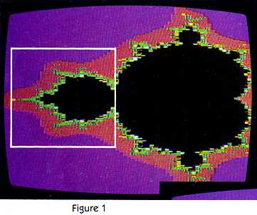
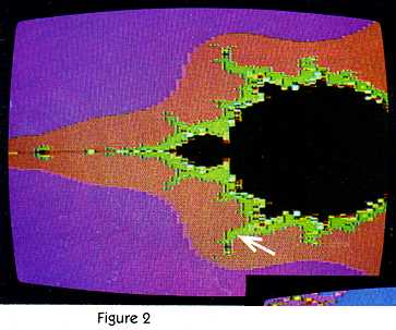
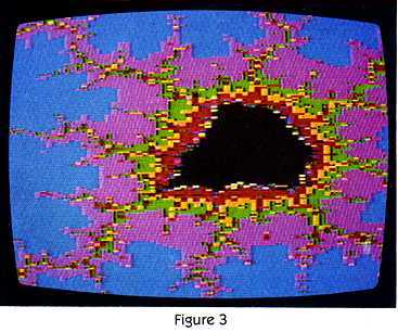
An entire Julia fractal curve is displayed in Figure 1. This is the image you get when you use the program's default data. Zooming in on the framed area in Figure 1 produces Figure 2. The result of several more zoom cycles is seen in Figure 3. The arrow in Figure 2 points to the area depicted here.
SELF-SQUARING
The algorithm used to create these images centers on an iterative process
called "self-squaring." This process, described in detail in the previous
article, is based on the formula:
![]()
Here, Z and u are complex numbers. Z represents
a point in the complex plane, u is a complex constant. Since
computers cannot work with complex numbers directly, we must write our
own complex number routines. These routines are in lines 320 and 330 in
the BASIC listing, and in the draw _fractal() routine in the C listing
for ST fractals appearing elsewhere in this issue.
If you're not comfortable with complex numbers, you can
think of self-squaring as a "black box." You put your Z value into the
top of the box, and two values come out of the bottom. One of these is
the new value for Z, the other is a measurement of Z, called Size.
Every point on the screen has its own unique Z value.
To process a point on the screen, we take its Z value and stick it into
our self-squaring black box. If the resulting Size value is less than two,
take the new value of Z, place it back in the black box and try again.
If Size remains less than two after 100 tries (or iterations), then the
point on the screen is inside the Julia curve, and should be colored black.
Points for which Size reaches two after 10 iterations, for example, will
have a different color. The color of a point depends entirely on the iteration
count.
THE MATH
In our complex number routines, AZ and BZ correspond to Z, a number
in the complex plane. AZ is the real part of Z, and BZ is the imaginary
part. Likewise, AC and BC correspond to u, the complex constant,
where AC is the real part of u, and BC is the imaginary part.
See this issue's Complex Numbers Introduction for more details.
Step 1:
The first step in self-squaring is to multiply Z by itself (hence the
term "self-squaring"). Since BASIC doesn't know how to deal with complex
numbers, we'll have to break each complex numbers into real and imaginary
parts, and separately process each part.
In this example, the complex value Z2 becomes:
(AZ + BZ)2 where AZ is the real part of Z,
and BZ is the imaginary part. This expression is equivalent to:
(AZ + BZ) x (AZ + BZ) and expands into:
AZ2+2*AZ*BZ+BZ2
An imaginary number can be expressed as a real number
multiplied by i, the square root of(-l). (In other words, i2 =
-1.) Since BZ is an imaginary number, squaring it yields BZ2
x i2, which is equal to BZ2 x -1, or -(BZ2).
And -(BZ2) is a real number.
Since AZ2 and BZ2 are both real
numbers, we can add them together to find the real part of our solution
to Z2. (Remember, BZ2 is a negative value, so we'll
be subtracting BZ2 from AZ2.)
We're still left with the 2* AZ * BZ term, which is the
imaginary part of our solution to Z2.
Step 2:
The second step in self-squaring is to add the complex constant u.
In our BASIC program, AC represents the real part of this constant, and
BC represents the imaginary part.
Once we've determined the real and imaginary values for
Z2, we simply add AC to the real part of our answer, and BC
to the imaginary part. Line 320 calculates the real part of our answer,
and line 330 calculates the imaginary part. These become the real and imaginary
values for our new Z.
We calculate the Size of our answer in line 350. The Size
of a complex number is equal to:
SQR(real part2 + imaginary part2)
If the Size of our answer does not exceed two, we take
our new Z value and put it through our self-squaring algorithm again. Keep
inserting each new Z value into the algorithm until its Size is greater
than two, or until we've been through the algorithm 100 times.
In the BASIC program, COUNT keeps track of how many times
we've been through the algorithm. If COUNT reaches 100, the corresponding
point on the screen is colored black. Other values of COUNT yield other
colors. In Fractal Zoom, COUNT may range between 1 and 101. The program
uses a series of formulas to convert COUNT into an appropriate color value.
These formulas lie in lines 1500-1550.
These formulas expect COUNT to range between 1 and 101.
Many times, however, COUNT will have a much smaller range. If we're zooming
in on a very tiny portion of the curve, for example, COUNT may only range
between 40 and 60. This range would only use the middle colors of our available
color spectrum.
If we know the maximum and minumum values of COUNT, however,
we can re-scale our color formulas to work over any range. To do this,
we must plot the entire Julia curve, remembering the maximum and minimum
COUNT values, modify our color formulas according to these values, then
re-plot the curve using the new colors.
To save a little time, we'll also store each COUNT value
in a disk file. This way, we only have to compute COUNT once for each point.
Once the program creates its new color formulas, it can retrieve the values
of COUNT from the disk file, instead of recomputing the entire curve. These
routines are in lines 502-508.
If you're plotting your curve in Graphics 8 (a two-color
mode), or if your COUNT values range between 1 and 101, the replotting
is not necessary and is skipped.
When the computer is done, your curve is saved to disk
as a 62-sector picture file. The data you used to create the picture is
also saved as a one-sector data file. The file used to store your COUNT
values is erased.
You'll need 62 sectors for the picture file, and up to
246 sectors for COUNT's temporary data file.
OVERNIGHT SUCCESS
This is why Julia curves take so much time (and disk space) to create
correctly. The computer must cycle through the self-squaring routine up
to 100 times for every point on the screen. That's from 15,360 points for
a GTIA screen to 61,440 points for a screen in Graphics 8 (ANTIC Mode F).
We've streamlined the program to increase its speed. For
example, we've removed the SQR operation from the Size routine in line
350. Now instead of comparing the square root of the variable SIZE to two,
we eliminate the square root operation, and compare it to four. The math
is the same, but we've eliminated BASIC's snail-paced SQR routine.
You may also want to turn off the display screen and the
ANTIC chip, which increases processing speed by up to 30 percent. If you
want to turn off ANTIC, answer N at the SCREEN ON (Y/N)? prompt. If your
screen is off and you want to take a glimpse of your "fractal curve-in-progress",
you can re-enable the screen display by holding down the [SELECT] key.
Once you release it, the screen will go black again.
If this is the first time you're using the program, you
should leave the screen on. This way, if a mistyped program line
causes the program to crash, an error message will appear. (Error messages
are invisible when the screen is shut off).
THE PROGRAM
Make sure you've got plenty of disk space before running the
program. Your picture file will require 62 sectors, and your temporary
data file will need between 123 and 246 sectors. When the program is through,
this data file will be replaced by a one-sector data file. This file will
contain the information the computer used to draw the curve.
When RUN, the program first asks whether you want to create
a fractal curve, or to load one from disk. Antic Disk subscribers will
find a ready-made fractal curve on the disk, under the filename D:JULIA.
CompuServe subscribers can find the same files in the
Atari 8-bit forum, Data Library 4, under the filenames JULIAl.XMO and JULIA2.XMO.
(Identical BIN versions are also available for TSCOPE users). JULIAl is
the 62-sector picture file, and should be renamed D:JULIA. JULLA2 is the
one-sector data file, and should be renamed DJULIA.DAT.
If you're running the program for the first time and you
don't have an Antic disk subscription or access to CompuServe, you'll have
to create a fractal curve from scratch.
CREATING A FRACTAL
When you choose to create a fractal curve, the computer will ask you
what graphics mode you'd like to use. Fractal Zoom can draw Julia curves
in Graphics Mode 8 (high resolution, two colors), Graphics 9 (medium resolution,
16 shades of one color), Graphics 10 (medium resolution, 9 colors), Graphics
11 (medium resolution, 16 colors of one luminance) and Graphics 15 (ANTIC
mode E, medium-high resolution, 4 colors).
Next, you'll be asked if you want to leave the screen
on during processing. Again, if you're using the program for the first
time, answer by typing Y.
Now, you'll be prompted for a filename for the completed
image. Make sure your filename does not have an extender! For example,
D:FRACTAL is an acceptable filename, but D:FRACTAL.PIC is not. If you enter
an improper filename, the computer will beep and reply BAD FILE NAME, and
then ask you for another filename.
Finally you should enter values for ACORNER, BCORNER and
SIDE. ACORNER and BCORNER are the real and imaginary Z values which correspond
to the upper-left corner of your screen. SIDE determines the magnification
value. Large values of SIDE yield smaller fractal curves, while smaller
values of SIDE yield larger images. If you don't know which values to use,
just press [RETURN] to use the default values printed at the bottom of
the screen.
The computer will plot the fractal curve, beginning at
the top left corner of the screen. When it's done, the computer will automatically
save the image to disk, and a DONE message will appear. Press [START] to
view the image and to begin the ZOOM routine.
DISK FRACTAL LOADING
You can load and zoom in on any fractal curve previously created with
this program. Just choose the LOAD ONE FROM DISK option and type in the
filename of the image to be loaded (no extenders allowed). The computer
will load the picture data. It will also examine the corresponding data
file to determine the graphics mode to be used and the values for ACORNER,
BCORNER and SIDE. Press the [START] key to view the image.
ZOOMING
Once you've created or loaded a fractal curve as described above, press
the [1] key, and a small frame will appear in the upper-left corner of
the screen. This is your zoom window. You can move the window with a joystick
plugged into port 1. You can vary the size of the window by pressing any
of the number keys (0-9). The [1] key will produce the smallest window,
and the [0] key yields a full-screen window.
Fractal Zoom will take the image within the zoom window,
and expand it to fill the entire screen.
Choose an appropriately sized window, move it over an
interesting portion of the Julia curve, and press the joystick button.
The screen will clear, and you'll be asked for a filename for your new
image. You'll also be asked whether or not you want the screen display
turned on.
This done, the computer will begin plotting your new fractal
image, starting at the top-left corner of the screen. When it's done, it
will save the picture and data to disk. You can continue zooming in on
an image almost indefinitely.
NOTES & HINTS
If you own a 130XE and are familiar with its RAMdisk, you can use it
to hold your temporary data files. Just change line 55 to read RAMDSK=
1 and your scratch files will be written to D8: but your picture file and
the permanent data file will still be written to a floppy disk.
Fractal curves are self-similar That is, the edge of a
fractal curve viewed at low magnification will look just about as jagged
as one viewed at high magnification. Until you become familiar with the
program and the Julia curve you're working with, you should only use the
larger zoom windows. When using the smaller zoom windows, it's too easy
to "get lost" inside an unfamiliar fractal curve.
Each time you zoom, you reveal curves and squiggles too
small to be seen previously When you use large zoom windows (lower magnifications),
you'll only see a handful of new squiggles. If you use small zoom windows
(higher magnifications), you'll reveal so many new squiggles that your
new image may be unrecognizable.
There are many Julia curves throughout the complex plane.
The one generated by the default data in Fractal Zoom is only one of many
possible curves. The more adventurous (and patient) users may want to enter
their own values for ACORNER, BCORNER and SIDE, and search for their own
Julia curves.
The most interesting parts of Julia curves seem to lie
in the filaments-the tiny "hairs" that appear to grow out of the body of
the curve. Zoom in on one of these for a special treat. And don't be surprised
if you discover a few miniature Julia curves hiding in these filaments!
(Kudos to any programmer who finds a way to replace the self-squaring loop-in lines 310-400-with one or two mathematic equations. The equations should accept variables AZ, BZ, AC, BC and return a COUNT value. An algebraic proof of the equations must also be submitted. The best solution, in the judgement of the editors, will be published in these pages. -ANTIC ED)
Listing 1 FRACTAL.BAS Download
Listing 2 LINES.BAS (not needed)
ON ANTIC Disk
JULIA.DAT Download
JULIA.MIC Download
ZOOM.DAT Download
ZOOM.MIC Download