Response Surface Mapping
New views for 3 -D graphics
BY JAMES PIERSON-PERRY
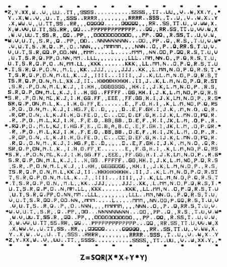
One of the more useful ways to study mathematical relationships is through graphics. Plotting a function usually gives a greater intuitive grasp of how the variables interact with each other. For example, a drawing of a sphere is much easier to comprehend than the function Z = SQR(R * R-X * X-Y * Y)
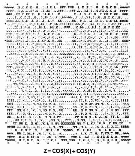
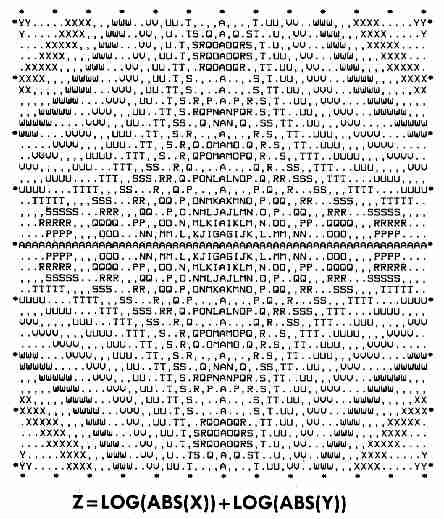
Response surface mapping is another way of representing 3-D functions and is widely used for scientific applications. These maps are also called "contour plots" because they resemble the contour lines on topographic land maps. RSMAP generates response surface maps for BASIC functions having one or two variables (X and Y). Analytical uses aside, many such graphs are interesting simply for their visual appeal.
In view of this, it is not surprising that 3-D graphics plotting is a popular software application. Examples of these include Paul Chabot's GRAPH 3-D (Antic, October 1985) for 8-bit Ataris, and Tom Hudson's CAD 3-D for the ST ($49.95. The Catalog, ST0214). Programs like these let you create, manipulate and print 3-D images of functions.
Response surface maps use colors or symbols to represent the Z (response) value, rather than plotting the third dimension in perspective. A weather map is a good example of a response surface map. Here, one type of symbol represents low pressure areas, while another symbol represents high pressure areas.
BACKGROUND
Most 3-D plotting programs give the illusion of three dimensions on
a flat surface. The resulting image is greatly dependent on the viewing
angle and may hide important parts of the function. Response surface mapping
programs always look "down" at the function, along the Z-axis. This gives
the entire X,Y grid as the viewing field.
The computer evaluates the function at each point on the grid and prints a letter corresponding to the resulting response value. We can extend this technique to examine functions having more than two variables. For example, consider the function Z=X*X+Y*Y+W*W We can make a separate map at various fixed values of W (called "slices") which, when viewed in sequence, give a good picture of what the overall function looks like.
THE PROGRAM
Type in Listing 1, RSMAP.BAS, check it with TYPO II and SAVE a copy
before RUNning it.
When RUN, RSMAP displays a title screen, then pauses and waits for you to type in your function. All standard BASIC arithmetic operators and transcendental functions are allowed. Constants such as P1 and E also may be used. You may define any of your own constants in line 1270. (NOTE: Embedded logic operators for discontinuous functions are not allowed.)
Here are some sample functions:
Z=X*X+Y*Y*PI
Z=LOG(ABS(X))+LOG(ABS(Y))/E
Z=ABS(COS(X)+COS(Y))
If BASIC detects any errors, you'll be asked to re-enter the function.
Next, enter the boundaries for the X and Y axes (even if only one variable is used) and the response limits. Estimates of the response minimum and maximum values are automatically generated to guide you in selecting the response limits. These limits will determine the resolution of the map.
Your Atari will now print the response map, along with a key to the response symbols. A typical map takes from two to five minutes to print. Press the [OPTION] key to abort the printout and enter new parameters.
Here are some additional interesting functions to get you started:
1. Z=LOG(ABS(X))+LOG(ABS(Y))
X,Y Ranges = -3 to 3
Z Range= - 6.5 to 2.5
2. Z=SQR(5-X*X-Y*Y)
X,Y Ranges = -1.5 to 1.5
Z Range = 0 to 2.5
3. Z=COS(X)+COS(Y)
X,Y Range = -3.14 to 3.14
Z Range = -180 to 180
PROGRAM TAKE-APART
The heart of the map processing is the short subroutine located at
the very start of the program to speed execution time.
Lines 1090-1190: Subroutine to evaluate the function over the X,Y grid and translate response values into map symbols. The symbols are stored in a buffer (B$) and printed one line at a time.
Lines 1240-1290: Initialize variables and strings. Current color register values are saved and restored at the end of the program.
Lines 1630-1800: Entry of the plotting function. We use the Atari's
"forced-read" mode to install the function into the program.
aside, many such
graphs are
interesting simply
for their visual
appeal.
Lines 1830-1890: Input X,Y boundaries and ensure the minimum value is less than the maximum value.
Lines 1910-2030: Routine to estimate minimum and maximum values of Z. A TRAP here prevents errors from illegal BASIC math operation, such as LOG(0).
Lines 2260-2410: Generate the response surface map.
Lines 2430-2510: Allow you to generate a new map using the same function but different ploting parameters.
NEXT STEP
Ambitious readers may want to modify this program to plot functions
on a graphics screen instead of a printer. Antic would be glad to see a
short, elegant enhancement which would support Graphics 15 (ANTIC Mode
E), Graphics 7 or any of the GTIA modes.
James Pierson-Perry of Elketon, Maryland is a research chemist with DuPont. His Molecular Weight Calculator program appeared in Antic, May 1986. Pierson-Perry was introduced to Atari computers in 1982 when his daughter's school began using them.
Listing 1: RSMAP.BAS Download