How Much Are You Worth?
SynCalc template figures it for you
A personal net worth file is a key document in planning your financial future. If you have SynCalc spreadsheet software and are familiar with its use, you can track your own personal net worth on an 8-bit Atari computer with at least 48K memory and disk drive.
How much are you worth? Net worth measures your financial growth and can help you attain desired financial goals. This file gives a projection for the next year, as well as each six-month period for the next two years. I use SynCale (Broderbund, $49.95) to update my net worth as ofJanuary 1 and July 1 each year. (We could not get this template to work with Calc Magic or VisiCalc. If you come up with a fix, send it to Antic for possible publication. --ANTIC ED)
To figure out your net worth, you need to know the value of your assets, liabilities and, in this case, liquid assets. Net worth is the dollar value of total assets minus total liabilities.
- Total assets = all money and property.
- Total liabilities = The sum of charge cards and other credit accounts.
- Liquid assets = cash in hand. In other words, available money--not including property.
ASSETS AND LIABILITIES
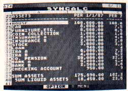
Sstart out by using your word processor to make a table of your assets and liabilities. Figure 1 shows the January 1, 1987 table for a fictional couple we'll call Tom and Betty.
Here, "property" includes all personal property--even if it's mortgaged or owned on borrowed money. For example: houses, furniture, automobiles, rentals, and valuable collections such as coins or stamps.
Tom and Betty own a house, furniture, a car and a coin collection. Except for the car, the market value for all this property will remain constant for the next two years. (The market value of the furniture is taken from the fire insurance policy.) Instead of using classified ads or a dealer's blue book, Tom established a car depreciation figure of $1,000 per year from his past history. The car cost $10,000 two years ago, and Tom thinks it will last eight more years.
Include the cash value, if any, of all insurance policies. Investments include stocks, bonds and limited partnerships. Note their current value and estimate the percent of increase based on past growth and dividend. Tom notes $3,000 of JB Inc. stock with a projected growth of 8 %.
Miscellaneous accounts are items not covered by other categories. Here, it's a one-year, $1,000 loan Tom made to his friend Bill at 6% interest.
The remaining items include Not Taxed Accounts and Taxed Accounts--only money earned in the taxed account must be reported at the end of the tax year.
Tom has three Not Taxed Accounts: two IRAs (Individual Retirement Accounts), and an account consisting of money contributed to Tom's pension by his employer. Tax on this must be paid upon retirement unless Tom puts it into another IRA. Every six months, $1,000 is added to each account. Interest averages 8%.
The Taxed Accounts are two savings accounts earning average of 8%, and a checking account earning 6%.
Once your assets are defined, list your liabilities--credit cards and all loans, such as home, car and rental property. Tom and Betty have a Visa card and two department store cards. Their current Visa debt is $2,000. Monthly payments are $80, and interest on the unpaid balance is 19%. Each store card charge totals $1,000. Monthly payments are $30 and interest is 19%.
Tom also has a one-year, $1,000 bank loan at 14.8% interest. He just applied for this loan, and is making the first payment. Tom's car loan is $8,000 at 12% interest for 48 months, and he's in month 24. The $75,000 house loan, 30 years at 10% interest, is in month 80.
Now we'll enter this raw data into SynCale and generate a personal net worth file. This article assumes that you already know how to operate SynCale software. For instance, you should know that pressing [OPTION] starts a command sequence, how to move around within the spreadsheet, etc. Keep your SynCale manual handy!
Antic Disk owners will find two complete templates on the monthly disk under the filenames NETJAN.SC and NETJULY.SC. You'll need to boot SynCalc before loading either of these files.
TYPING THEM IN
Even if you're a SynCale whiz, please pay close attention to these instructions--and carry them out in the exact order printed here. There is difficult typing ahead, with no TYPO II to help you.
Immediately after booting SynCalc, place a blank disk into your drive. Format this disk using the FORMAT function from the LOAD/SAVE menu. (Don't use the FORMAT function from the COMMAND menu!) Next, set all your column widths to seven. Press [ESC] to remove the command bar and type: /FGW 7
Now, type /FGP 2 to set GLOBAL FORMAT PRECISION to two. When the PRECISION function is set this way, all of your dollar values will be rounded to the nearest cent.
Type /FG, to enable the COMMAS function: When chosen, this function will insert commas in numbers like 1,000. Next, type /RM to enable the GLOBAL RECALCULATE MANUAL command. This function speeds data entry.
Type /FL A1:A255 ta justify your entries in column A against the left margin. Type /FR F1:H255 to justify your entries in columns F through H against the right margin. Finally, type /RR to set calculation to ROWS.
You're now ready to type in the spreadsheet information. Copy the text headings shown in Figure 2 into column A of your net worth template. If a title exceeds seven characters, type it in anyway--SynCalc's overflow feature handles the over-long material automatically. (But you need to erase each overflow cell manually if you move the title.)
Figure 2 shows a completed NETJAN.SC template that gives you Tom and Betty's net worth, total assets, total liabilities and liquid assets on January 1, 1987 and as projected for every six months during the next two years. This Tom and Betty sample file is intended simply as a guide that you can adapt to your own situation!
You must enter all numbers and formulas in the cells shown, or else the template won't work. Enter zeros in columns B to E to "hold open" the cells for formulas and values to come later.
Listing 1 shows each cell address, followed by the entry. Don't type the cell addresses (such as D7) shown in the first three or four spaces at the left. Instead, type /Gcellname to go to that cell. /GD7, for example, puts your cursor at cell D7. Once you're at the cell, type in the formula, typing over the space holding zeros entered earlier.
A formula element like E17 is not text--type it as +E17 so that SynCalc will know it's a numeric entry. As you enter each formula, protect it by typing /FO (FORMULA PROTECT ENTRY) so you won't accidentally write over it.
TOM AND BETTY
Enter Tom and Betty's yearly interest projection in cell D4. Try changing the interest rate and seeing the impact of a new projection. Tom shows 8%, based on a review of the interest data in Figure 1-- six line items of 8%. Tom could also enter the three credit card interest rates (19%) into nearby cells. Next, enter the Figure 2 loan data between cells D6 and F14. If you have more loans than shown in the example, just repeat the procedure until you're done.
After typing in the text as shown in cells D6 through D14, Tom enters "house" under column E. The loan is the initial amount borrowed ($75,000). The interest is entered as a decimal (0.10). Enter the number of monthly payments (360) and type the current payment number (80) in the line below.
The monthly payment amount (PAY/MONTH) goes in the cell below. Tom used this formula for the monthly payment of the house loan in cell B9:
B5/((1-(1+ B6/12)^ -B7)/(B6/12))
(The ^ -B7 is not a misprint. It means you 're raising the value of B7 to a negative power. This is the same as ^(1/B7).--ANTIC ED)
For the car loan, use B12, B13 and B14 instead of B5, B6 and B7. The last item, cells B10 and B17, is the interest rate factor. Here's the formula for B10:
((1+B6/2)^(1/6)-1)
For B17, substitute B13 for B6 in the formula.
Rate factors for the other loans are calculated the same way. Just make sure that the cell letter is the same as the column letter for that particular loan.
Now enter the current value data for assets and liabilities. Move to the equivalent of row 24 shown in the example. Enter the text data in column A from the data you generated that is similar to Figure 1. Do the same for column B. Remember, when compiling the asset and liability data, we calculated the current value for the house and car loans while preparing the net worth file in Table B cells B48 and B50.
Tom used this formula for his house and car loans. (The house loan is in column E and the car loan in column F.):
B9*(1-(1+B6/12)^(-B7+B8))/(B6/12)
The house and car loan equities are easy to calculate. The loan equity equals the amount of the loan minus the value of the above formula.
PROJECTED DATA
Move to the equivalent of cell C24 in your file before inserting the projected data shown in columns C through F. Figure 1 indicates a constant market value for the house, furniture, coins and insurance for both Betty and Tom, so he copied the cell B24 current house value into cells C24, D24, E24, and F24 by typing B24 into each of these cells. If cell B24 is changed, all corresponding cells to the right of B24 would change also. Tom also did this for furniture, coins and insurance.
Due to car depreciation, the cells to the right of B25 were treated diffently. In Figure 2, Tom entered the value B25-500 into cell C25, C25-500 into cell D25, D25-500 into cell E25, and E25-500 into cell F25. Therefore, each cell reflects a depreciation of $500 compared to the cell to the left. A change in cell B25 instantly revises all neighboring cells.
To accommodate the constant 8% annual interest for JB Inc. stock, Tom entered the following formulas into cells C30, D30, E30 and F30:
B30 * (1+ C4/2)
C30 * (1+ C4/2)
D30 * (1+ C4/2)
E30 * (1+ C4/2)
Bill's loan was handled differently: the interest was deducted from the initial loan at the start ($1,000- (.06 *1000)), and the balance ($940) was divided into 12 payments of $78.33 each. Therefore, Tom entered 940 in cell B31, B31-(940*F6/12) in cell C31, and C31-(940 * 6/12) in cell D31. The zero in D31 means the loan has been paid, so he entered zero into cells E31 and F31.
The values in rows 35 through 39 all use the same formula -except the identification of the row number of each cell is different. For cells C32, D32, E32 and F32 the formulas are:
(B32+1000)*(1+C4/2)
(C32+1000)*(1+C4/2)
(D32+1000)*(1+C4/2)
(E32+1000)*(1+C4/2)
The cells in row 35 are handled as above, except 1200 is used instead of 1000 because of the difference in the amounts deposited every six months. The checking account entry is B37 * (1 + 0.06/2) for cells C37, D37, E37 and F37.
The assets data is completed after entering the the assets (the sum of the columns from row 24 through row 37: @SUM(B24:B37)) and liquid assets (the sum of columns from rows 32, 33, 35, 36 and 37).
The formulas used to calculate the projected six months for the Visa and two department store accounts is lengthy. Since the net worth file indicates trends and doesn't have to be accurate to the nearest dime, Tom used this formula :
(B-(P*6))*(1+R/2)
B Is the balance shown in the cell to the left, R is the interest rate and P is the monthly payment. For example, cell C49 says:
(B46-(30 * 6))*(1 + .19/2)
Tom's formula for the cells showing the bank loan projection is the balance shown in the cell to the left minus the amount paid each month. It's calculated like this:
1000-(.148*1000)=$852.
Put 852 into cell B48. For cell C48 this is B48-(71*6), and for cell D48 this is C48-(71 * 6).
Since Tom didn't have the current balance for the house and car loans (see Figure 1), he calculates the current balance and projected value for them. Here's the formula for cell B49:
B9*(1-(1 + B6/12)^ (-B7 + B8))/(B6/12)
B8 shows the current payment number of the house loan. For cell C49 this value is B8 + 6, since it's for a time period six months later. For cell C49 the above formula is:
B9*(1-(1 + B6/12)^ (-B7 + B8 + 6))/(B6/12)
For the automobile loan, use row 50 and replace B5 through BI0 with B12 through B17.
Finding the sum of the liabilities is like finding the sum of the assets. Here, it's the sum of all of the columns from rows 45 through 50.
You'll finish the net worth file after entering the formulas into cells 129 through 148. Enter total assets into cells 134 through 138 (@SUM B39:F39). Also, enter the total liabilities and liquid assets from the cells in rows 40 and 52. Finally enter the formulas into cells 129 through 132. For example, into cell 129 enter the formula for the current net worth: B39-B52. This logic applies to the remaining net worth cells; total assets minus total liabilities for the same time period.
UPDATING
Every attempt was made to make sure each cell uses the data in the cell to its left. This simplifies the updating of the net worth file. For example, when a value in column B is revised, the remaining cells in that row change automatically.
For example, Figure 3 shows NETJULY.SC, the updatad file for July 1, 1987. First, Tom changes the current date shown in cells I29, 134, 133 and I44 to JUL 1, 1987. Next, he adds six months to the current loan payment number for the house and car loans (shown in cells B8 and B15) to 86 and 30 respectively.
Then Tom revises the dates shown in rows 22 and 43. Column B reads "PER 7/1/87". Six months will be added to the remaining columns so that "PER 7/1/87" will appear in column F.
The Projected data for 7/1/87 shown in column C is revised and compared with the actual value for this date. For example, the current value of the house remains the same, as do the values of the furniture, coin collection and both insurance policies.
The new value for the car, $7,500, goes in B25. All remaining cells in this row reflect this new data input. The JB Inc. stock does a little better than Tom predicted, let's reset its value at $3,285. However since Tom believes that the projected 8% interest is still valid, he puts 3285 into B30.
Bill's loan repayment proceeds on scedule, so Tom types 470 into cell B31. The IRA accounts, company pension, and bank accounts are at the projected values, so Tom enters the values shown in cells C32 to C36 into the respective cells in column B. The checking account is lower than projected--only $963--so this value is entered into B37. All of the assets, including the sum of the assets and the sum of the liquid assets, automatically change.
Any new assets are entered into the file in their proper places between the current entries. The spreadsheet should automatically accept any new or deleted entry and readjust the resulting expressions in the remaining cells.
The current values for the Visa, credit card and bank loans are entered in column B. Here, Tom's projected values were correct and the values in column C go into the respective cells in column B. The house and car loan entries are revised automatically by the changes in cells B8 and B15.
The net worth file is now ready for you to examine and analyze, this year and for years to come. Some experts believe your net worth should show an annual growth of about 10%.
SYNCALC
Broderbund Software
P.O, Box 12947
San Rafael, CA 94913
(415) 479-1185
$49.95, 48K disk
Gordon Toomey is an aerospace engineer from Rancho Palos Verdes in Southern California.